Neural Radiance Fields (NeRF) Tutorial in 100 lines of PyTorch code
Neural Radiance Fields (NeRF) is a hot topic in the computer vision community. It is a 3D scene representation technique that allows high-quality novel view synthesis, and 3D reconstruction from 2D images. Its widespread use in the industry is evident through the increasing number of job advertisements by big tech companies seeking NeRF experts.
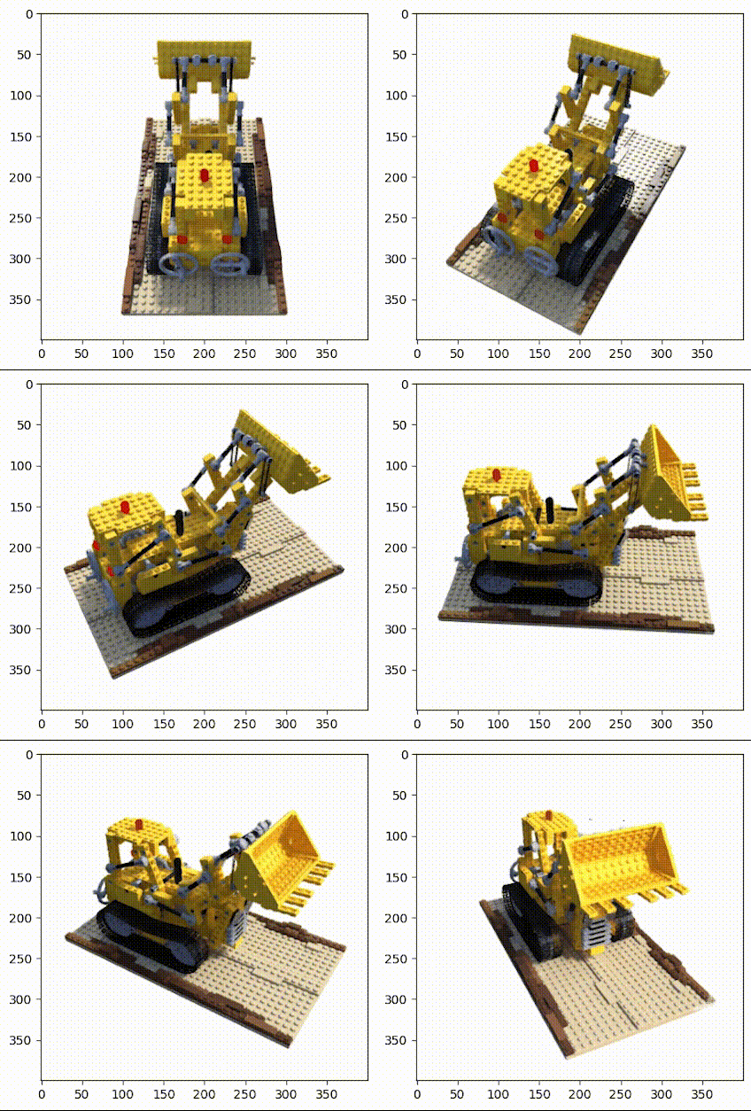
In this tutorial, we will implement the initial NeRF paper from scratch, in PyTorch, with just 100 lines of Python code. While simple and concise, the implementation will provide the nice results below.

This tutorial primarily focuses on the implementation and does not delve into the technicalities behind each equation. If there is interest, this information could be covered in a separate article. In the meantime, for those who wish to gain a comprehensive understanding of the technology and advancements made since the initial 2020 paper, I have a 10-hour course available on Udemy that covers NeRF in detail.
Rendering
A key component in Neural Radiance Fields, is a differentiable rendered that maps the 3D representation represented by the NeRF model into 2D images. Then, the problem can be formulated as a simple reconstruction problem

where A is the differentiable rendered, x is the NeRF model, and b are the target 2D images.
In short, the rendered takes as input the NeRF model together with some rays from the camera, and returns the color associated to each ray, using volumetric rendering.
The initial portion of the code uses stratified sampling to select 3D points along the rays. The Neural Radiance Fields model is then queried at those points (together with the ray directions) to obtain the density and color information. The outputs from the model can then be used to compute line integrals for each ray with Monte Carlo integration, as outlined in Equation 3 of the paper.
The accumulated transmittance (Ti in the paper) is computed separately in a dedicated function.
Nerf model
Now that we have a differentiable simulator that can generate 2D images from our 3D model, we need to implement the model itself.
One may expect the model to have a complex structure, but in reality, NeRF models are simply Multi-layer Perceptrons (MLPs). Yet, MLPs with ReLU activation functions are biased towards learning low-frequency signals. This presents a problem when attempting to model objects and scenes with high-frequency features. To counteract this bias and allow the model to learn high-frequency signals, we use positional encoding to map the inputs of the neural network to a higher-dimensional space.
Training
The implementation of the training loop is straightforward, as it involves a supervised learning approach. For each ray, the target color is known from the 2D images, allowing us to directly minimize the L2 loss between the predicted and actual colors.
Testing
Once the training process is complete, the NeRF model can be utilized to generate 2D images from any perspective. The testing function operates by using a dataset of rays from test images, and then generates images for those rays with the rendering function and the optimized NeRF model.
Putting it all together
Finally, all the pieces can be easily combined. In order to keep the implementation short, the rays are encoded in a dataset which can be loaded. If you want to learn more about the ray computation, I invite you to have a look at this code, or to follow my course on Udemy.
I hope this story was helful to you. If it was, consider clapping this story, and do not forget to subscribe for more tutorials related to NeRF and Machine Learning.
[Full Code] | [Udemy Course] | [NeRF Consulting] | [Career & Internships]
